SIMPLE NEURAL NETWORK WITH C++

This project focuses on artificial neural networks. The objective is to design and implement a simple neural network model to perform a basic classification task, utilizing training data obtained from Kaggle. The dataset used to evaluate the model's performance pertains to fraud detection. It consists of several anonymized features, and the model is tasked with predicting whether a given input instance, represented by these features, should be classified as a positive (fraudulent) or negative (non-fraudulent) case.

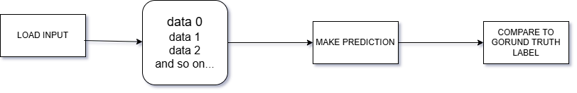
In simplified terms: a dataset x is input into the model → the model processes the input → generates a prediction → the prediction is compared against the ground truth label.

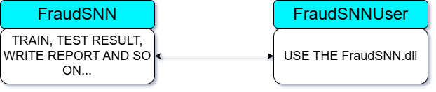
All tasks will be encapsulated in a project named FraudSNN. This project will produce a final output in the form of FraudSNN.dll. If asked why a DLL is used, the reason is that the entire project will be written purely in C++ from scratch, without any third-party libraries, in accordance with the primary goal of this project: performance.

In addition to performance considerations, a DLL also supports access from various areas of the programming world. As long as it is accessed from Windows, the support and applicability of using this DLL file will be broader in scope.

FraudSNN will include several essential features for model training and development. However, the fine-tuning and other testing processes leading to optimal results will not be shown, as detailing these steps chronologically would make the project excessively long. Nevertheless, I will still explain that FraudSNN.dll is capable of performing such tasks and supporting various aspects of model development, though I will not elaborate in detail on how I arrived at the configurations that produced relatively high prediction accuracy.

In general, the main functions provided by this simple neural network will include: reading data, training on the data, generating reports (note that some specific practical uses of this function will not be documented, although they are certainly used by me to achieve relatively high prediction accuracy), saving the learning results in the form of weight and bias configurations, creating model configurations, and loading both model configurations and previous training results.

If a DLL can be considered a universal Windows library, then it is also necessary to create a program to test the execution of this DLL file. Therefore, an additional project will be developed to test FraudSNN.dll, and this project will be named FraudSNNUser.

FRAUD SNN (SIMPLE NEURAL NETWORK)

The FraudSNN project is essentially a simple neural network project. In other words, this project can also be used to train on datasets other than the fraud data we will use for testing this time. However, it is important to note that this project is intended solely for basic classification tasks. Remember: this is a simple classification neural network.

Four .cpp files will be created for the FraudSNN project, each responsible for handling a specific component:

neuralNetwork.cpp
mathF.cpp
vectorOrganizer.cpp
fileOrganizer.cpp

Each of these .cpp files will be accompanied by their corresponding .h header files to facilitate interconnection. However, neuralNetwork.cpp will be specifically designed to interface with external programs. Therefore, neuralNetwork.h will only contain the functions intended to be exported into FraudSNN.dll for external program interaction. Meanwhile, mathF, vectorOrganizer, and fileOrganizer will serve solely to provide internal functionalities required by neuralNetwork.cpp as the main execution module.

The mathF file, as its name suggests, will provide the mathematical functions needed. vectorOrganizer will handle functions related to vector operations, while fileOrganizer, as the name also implies, will be used for managing file-related operations.

mathF.cpp

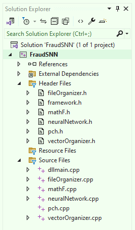
Please disregard components such as pch, dllmain, and other files unrelated to the four .cpp files and their corresponding .h files mentioned earlier, as those are default files automatically generated when creating a DLL project in Visual Studio.

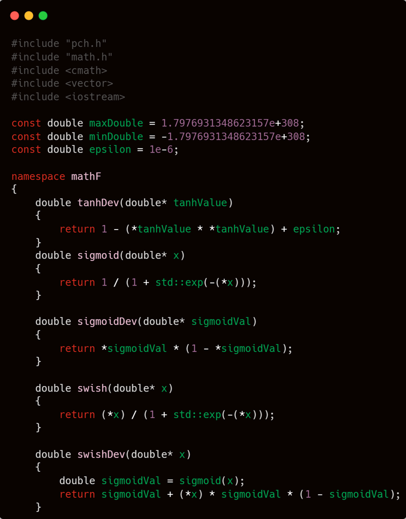
Mathematics is the fundamental foundation of artificial intelligence. Therefore, it is the first aspect that must be considered in AI development—whether the system is simple, complex, or moderate in nature. Prioritizing the mathematical component is a wise and essential step.

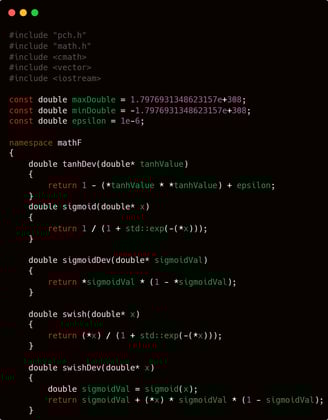
For simple mathematical components such as basic activation functions and their derivatives, I will not provide lengthy explanations, as I believe it is unnecessary. After all, they are merely a set of basic arithmetic operations with a touch of elegance—there is nothing that truly requires detailed explanation.
I will provide three activation functions along with their derivatives for the hidden layer.

Hyperbolic tangent.
Sigmoid.
Swish

Before dealing with the functions required in mathF.cpp, it is best to first define the namespace that will encapsulate them, along with several constants that may be needed in those mathematical functions.

I will wrap the functions to be created within the mathF namespace, and I will also define three constants commonly needed in basic mathematical operations: maxDouble, minDouble, and epsilon.

maxDouble and minDouble, as their names suggest, will be used to store the maximum and minimum values that a double type can hold. These are typically needed in functions that compute the maximum or minimum value within a vector. Meanwhile, epsilon is commonly used to prevent computations from producing invalid values—ensuring numerical stability by substituting extremely small values where necessary.

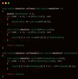
With three activation functions for the hidden layer, the choices become more varied. However, for the output layer, I will provide only one activation function: softmax.
I chose softmax, of course, because it is particularly well-suited for classification tasks.

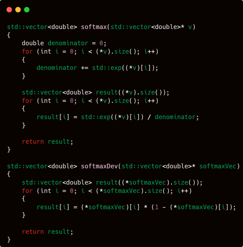
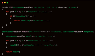
And as for the loss function—perhaps you’ve already guessed it. Who else if not the one and only, the esteemed CCE (Categorical Cross Entropy).

If observed in more detail, the CCE function I wrote may appear a bit unusual and not entirely identical to its mathematical definition. Instead of computing the sum of target * log(predicted value), the CCE function I designed returns only the value of -log(predicted value corresponding to the class with a value of 1 in the target vector).

This is essentially a double-edged sword. If the class with a value of 1 in the target vector is located at the beginning of the vector, the function will return a result more quickly; however, if the value 1 is located near the end of the vector, the function will return a result more slowly.

But regardless of that, CCE is ultimately just a metric for measuring the progress of a model during training. Furthermore, I actually disagree with using CCE as the success metric for a classification model. Why? Because, in my view, what truly matters is the model's accuracy in making predictions. So, if the program can predict more than 90% of the given samples correctly, who cares about the CCE value?

The next two functions are getOneId and getValueMaxId. getOneId is used to retrieve the index of the target class that has a value of 1, while getValueMaxId is used to obtain the index of maximum value from a vector.

Both of these functions will be used later in the context of backpropagation. I will not explain them in detail for now, but the main point is: please understand the purpose of these two functions first, as they will be relevant in the upcoming explanations once we enter the backpropagation phase in the neuralNetwork.cpp file.

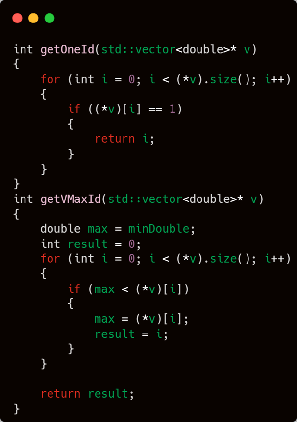
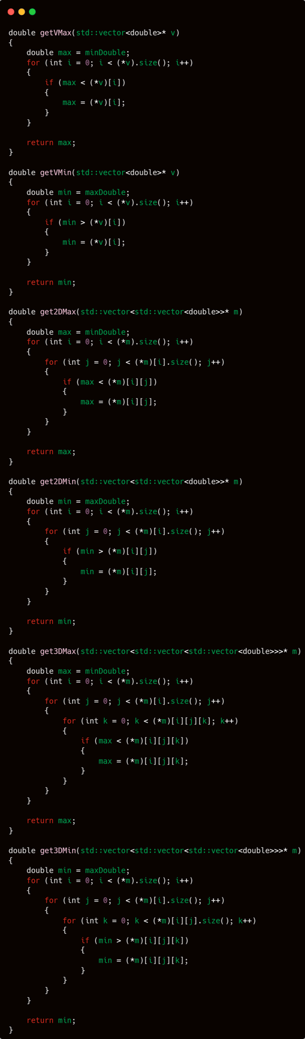
Remember the two constants defined earlier—maxDouble and minDouble? These two constants are used in the following two functions: getVMax and getVMin. getVMax is used to obtain the maximum value from a vector, while getVMin is used to obtain the minimum value from a vector.

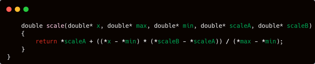
These two functions will be used frequently. One example of their usage is within the scaling function, which is designed to transform all values in a vector to a specific range.

The constants maxDouble and minDouble are also used to obtain the maximum and minimum values from multi-dimensional vectors. In this case, I have implemented the functionality up to 3-dimensional vectors.

And the final function in the mathF namespace is the scale function. This function transforms a set of numbers into a specified custom range.

fileOrganizer.cpp

Unlike mathF.cpp, which is more focused on mathematical operations, fileOrganizer will concentrate more on actual programming—specifically, programming tasks related to reading from and writing to storage media. As the name suggests, it is a file organizer: organizing file operations.
And just like the previous file, the functions in fileOrganizer are wrapped within a namespace—specifically, the FO:: namespace.

The first two functions I will discuss are among the most crucial ones. They have both been used and are confirmed to work. However, one of them was not demonstrated in practice because I used it in a context unrelated to testing whether this program can train a simple neural network or not. As I promised earlier, I will explain their purposes and guarantee their functionality—in the sense of technical correctness.

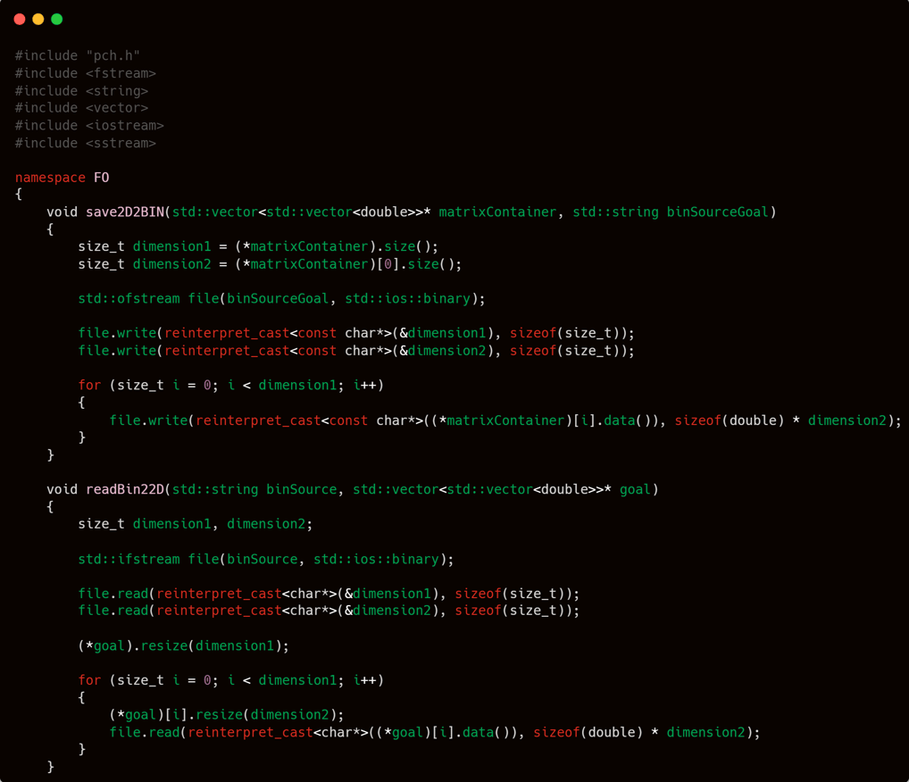
Pay close attention to the two functions above: void save2D2BIN and void readBin22D.

In short, the save2D2BIN function is used to save a two-dimensional vector in the form of std::vector<std::vector<double>> into a binary file, while readBin22D serves to read that file back.

Writing and reading files in binary format may seem trivial and unrelated to a model’s success in learning a pattern. But believe me—when the input itself consists of hundreds of thousands or even millions of rows, each containing numerous features, reading a plain text file like a .csv can take an extremely long time. As a result, refinement processes such as fine-tuning—which frequently access the input file—will take significantly more time if the file is not in binary format. And besides, what’s wrong with making file reading much faster, right?

Wait a moment, I will present two more functions that I will use in collaboration with these two, forming a stronger synergy. Please be patient.

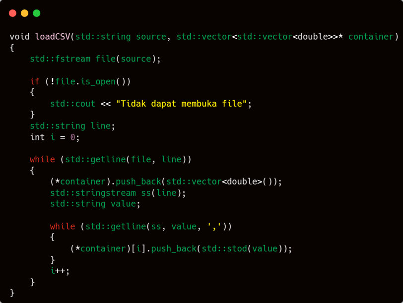
loadCSV is a simple function: read a text-based file using "," as the delimiter → read it line by line and store each line → split each line based on the delimiter "," and convert each value into a double type → append it to the result vector → Simple, right?

Now let’s move on to the combination factor, just as I previously promised.

The combination I’m referring to is converting input originally in .csv format into .m, which is a binary file. The process is quite simple: load the .csv file using loadCSV → store it into a vector container → write the vector container into a .m file using save2D2BIN.

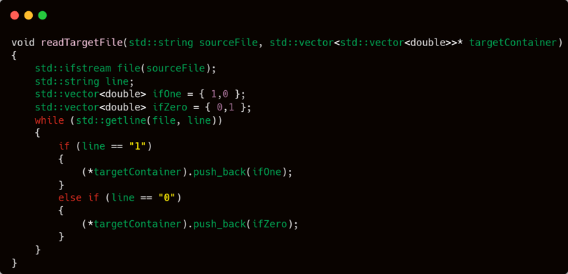
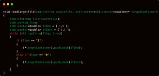
Next is the readTargetFile function. You might wonder, why not just use loadCSV to read the file? Well, in some cases, CSV files are written in a line format like
"0,0,0,1,0,0,0"
However, for this task I created a dedicated function because it's purely a binary classification task. The job is simply: "predict whether this is a fraudulent transaction or not based on the input from training row x." In other words, it’s just binary classification. That’s why I created a custom method for reading target labels specifically for this kind of binary classification setup.

The way it works is by checking whether the file contains a 0, which means a negative (non-fraudulent) transaction, or a 1, which indicates a positive (fraudulent) transaction. If a 1 is detected on row x, then simply append a one-dimensional vector in the form {1, 0}; if a 0 is detected, append a vector {0, 1} to the two-dimensional target list matrix.

The next four functions I will write are for reading and writing network configurations. These functions form the core foundation for saving and loading the learned parameter configurations. Weights and biases are stored and retrieved using these functions.
If asked why I don’t save them in .csv format, the answer remains the same as why I converted the input from .csv to binary files: speed.

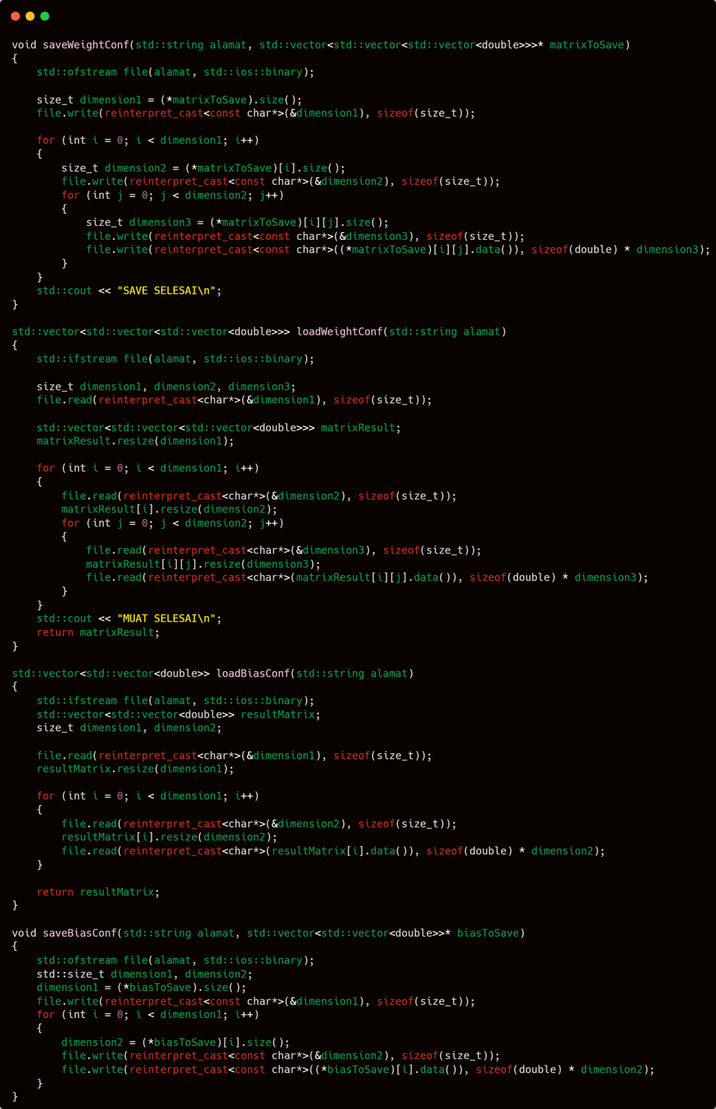
Indeed, they are four different functions, but the core principle behind them remains the same.
The key to saving a multi-dimensional matrix is to include both the dimension sizes and the values held by each element within those dimensions.
This is quite similar to the save2D2BIN function we discussed earlier. However, the difference is that save2D2BIN is used to store input or a table with a predefined size.

Why don’t we just use save2D2BIN to store, say, biases? The answer is simple: because biases are not shaped like a flat table. In a flat table, if it’s declared to have 10 rows and 10 columns, then every row has exactly 10 columns. That structure contradicts the nature of biases, which—even though they are also two-dimensional—are not flat.

For example, if a network has 3 hidden layers, each with 2 nodes, and an output layer with 10 nodes, then clearly the structure is not flat. Saving the biases for the hidden layers alone could be flat—since there are 3 layers with 2 nodes each, it forms a 2×3 matrix. But since the output layer (which is part of the network) has 10 nodes, the overall bias structure becomes 2×3 + 10, which breaks the flat matrix shape.

Therefore, the writing method must also be adjusted. While saving a 2D table only requires storing the dimension sizes and the element values, in this case, the elements of each dimension must be recorded individually—since the first dimension may not have the same number of elements as, say, the tenth or any other.

So the basic mechanism is as follows:
First, store the size of the outer dimension. Then, before writing the collection of values that belong to a specific inner dimension, record how many elements that particular dimension contains. This ensures that when reading the binary file later, the byte range for each segment remains valid and is not exceeded.

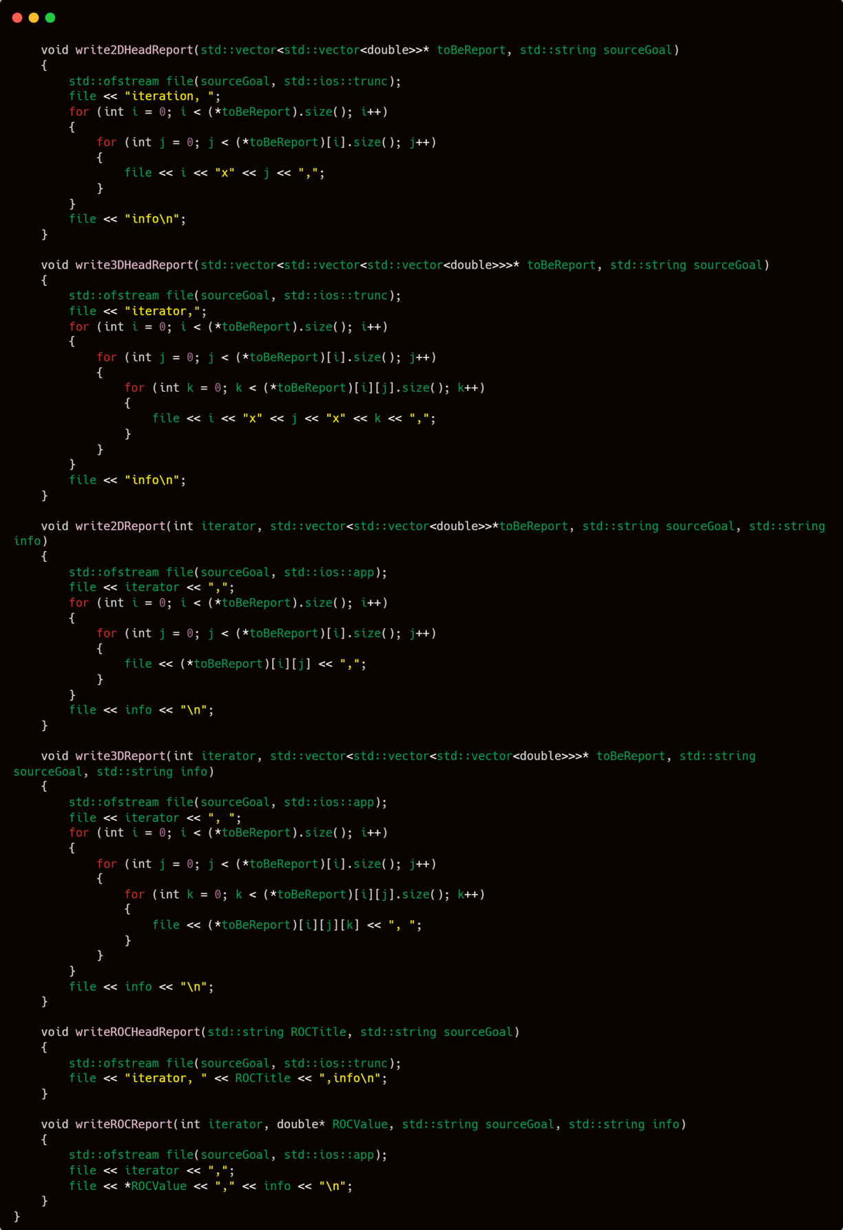
The final functions I will prepare under the fileOrganizer category are a collection of logging functions—functions specifically designed for recording reports or logs of the neural network’s activity and progress.

There are three pairs of logging functions I will prepare:

2D Report Logger
Used for recording two-dimensional data (e.g., weights of a single layer or performance metrics across epochs).
3D Report Logger
Useful when logging data that changes over time across multiple dimensions (e.g., weights across several layers and epochs).
ROC Logger (Rate Of Change)
Specifically tracks the change in a single value over time—ideal for monitoring metrics like loss, accuracy, or any scalar parameter that evolves during training.

These logging functions are essential not only for analysis and debugging but also for understanding the behavior and development of the neural network over time.

I won’t demonstrate the usage of all these logging functions directly. However, I will explain several scenarios where each of them should be used and how they are expected to help resolve specific challenges:

🔹 2D Report Logger – For Layer-specific Snapshots

Use Case:
When you want to record the change of bias vector after certain training operation (e.g., everytime after backpropagation).

Why it helps:
This provides insight into how the parameters of a specific layer evolve, which is useful for diagnosing issues like vanishing gradients or overfitting at certain layers.

🔹 3D Report Logger – For Multi-layer & Epoch Tracking

Use Case:
When tracking weights or biases across multiple layers over multiple epochs, especially in deeper architectures.

Why it helps:
You can later visualize or analyze trends in how each layer adapts over time—valuable for identifying bottlenecks or underperforming layers.

🔹 ROC Logger – For Monitoring Change Trends

Use Case:
To log the change in loss, accuracy or max output value over time.

Why it helps:
You can detect plateaus, divergence, or instability during training. This logger is especially helpful for fine-tuning learning rates or early stopping decisions.

Even though not all of them will be directly practiced, knowing when and how to use these functions is very important. This will help keep the training process healthy and well-directed—especially as the network grows more complex.

vectorOrganizer.cpp

vectorOrganizer.cpp — Unlike the two previous .cpp files that contain many complex and intricate functions, vectorOrganizer is likely the simplest and easiest group of functions to understand among all the other .cpp files.

Why is that?

Because the vector library — being a standard C++ library — already provides a wide range of built-in functionalities, leaving little need for custom-built operations from scratch.
Even some of the functions here might exist solely to shorten code, avoiding repetitive and complex writing. From a functionality standpoint, they may not bring any significant advancement.

However — regardless of that — these functions still play a helpful and supportive role in the development process.

Without further ado, let’s jump straight into the first function.
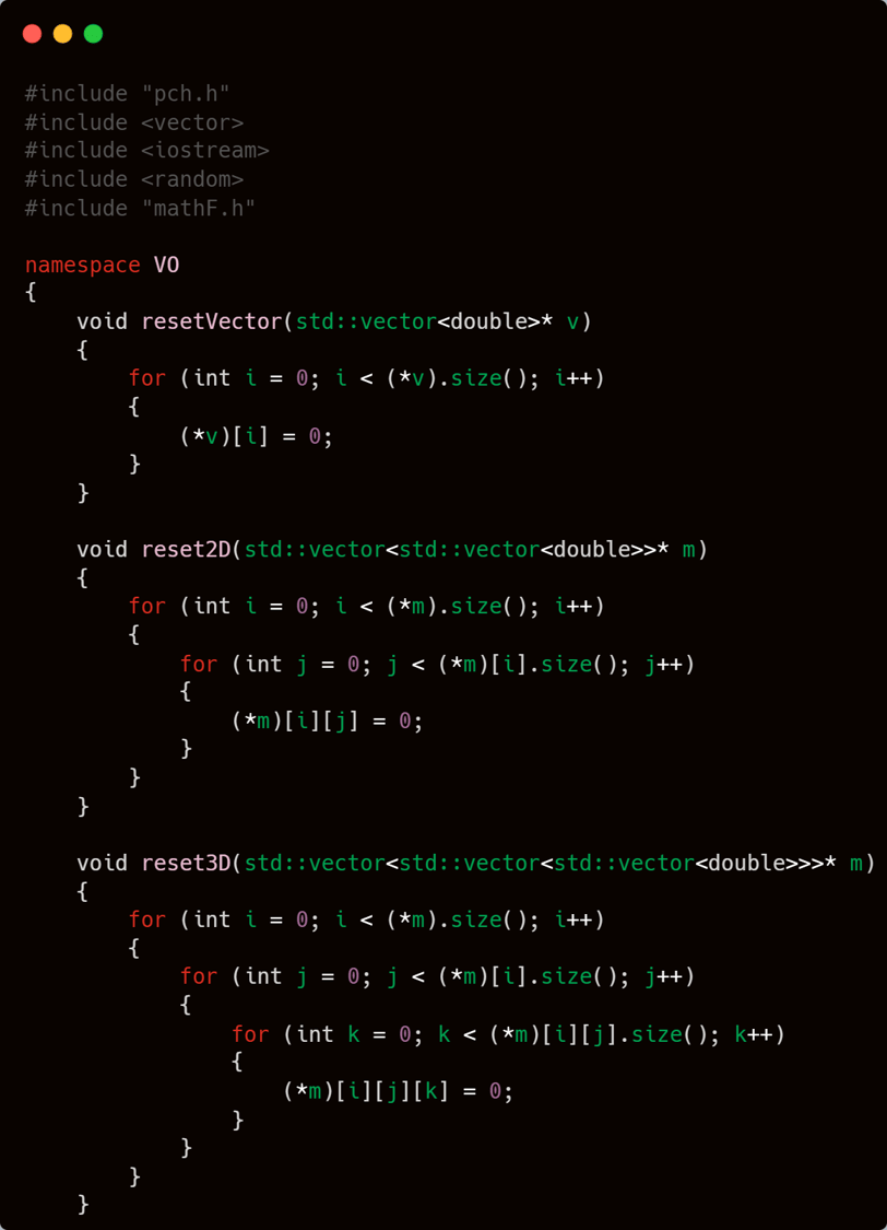
Unlike other .cpp files, vectorOrganizer.cpp contains fewer functions, making it more lightweight in comparison. The first function I’ll discuss is about resetting vectors or matrices.

This function is essential when you want to:

Clear the contents of a vector or matrix.
Reuse the structure without re-allocating memory.
Reset all values to zero or another default value for the sake of initializing a clean state—common in training loops or forward/backward propagation steps.

While it may seem trivial, having a dedicated reset function improves code clarity and consistency across modules.

Most of the vectors used in this program are 3-dimensional down to 1-dimensional. Although later there will be a 4-dimensional vector, but we will discuss that later. For now, let's focus first on operations on these 3 vector forms.
Reset vector, as referred to here, simply means changing all the values stored in the operated vectors to zero. Yes, it's that simple — just set the values stored in the vector to 0. So, whether it's 2-dimensional or 3-dimensional, the essence remains the same:

Set all the values stored in the given vector or matrix to 0. Done.

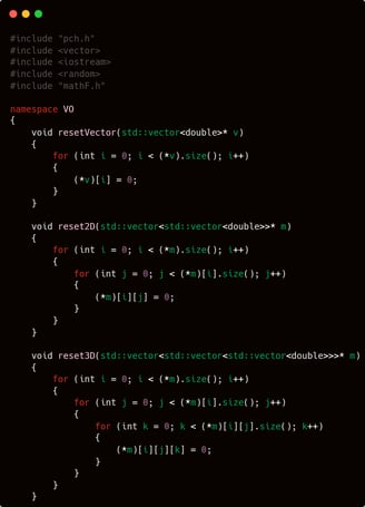
Once the reset vector function is available, let’s proceed to create the print vector/matrix function.

📌 The goal of this function is to display the contents of a vector or matrix — whether it's 1D, 2D, or 3D — in a readable format, which is especially helpful during debugging or manual inspection.

Let’s move on to implementing these print functions, one for each dimensional type.

Indeed, printing vectors or matrices can be very helpful during fine tuning. However, I strongly recommend minimizing the use of these print functions. Why? Because unless there’s a specific purpose — like monitoring the progress of weights, biases, or other parameters at certain iterations — it’s better to avoid it, since printing consumes quite a heavy amount of computation.

I won’t be practicing their usage extensively, but I guarantee these print functions work reliably and correctly.

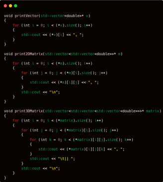
Next up are two functions that I will definitely use because they are crucial in building an artificial neural network model. These two functions are:

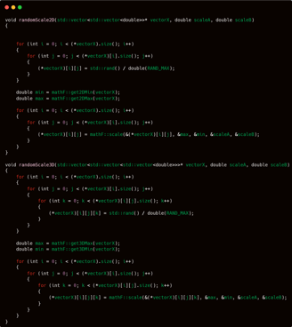
randomScale2D
randomScale3D

They are responsible for randomly scaling matrices in 2D and 3D forms, which is essential for initializing weights or biases with random values within a specified range.

This function essentially just creates an access space that will later be used to scale the values stored inside the parameter vector or matrix. So, yes — the main work actually happens in the mathF namespace.

The key functions called within these are to:

Get the maximum value
Get the minimum value
Pass the value x to the scale function from the mathF namespace

These are the core operations always invoked inside these scaling functions.

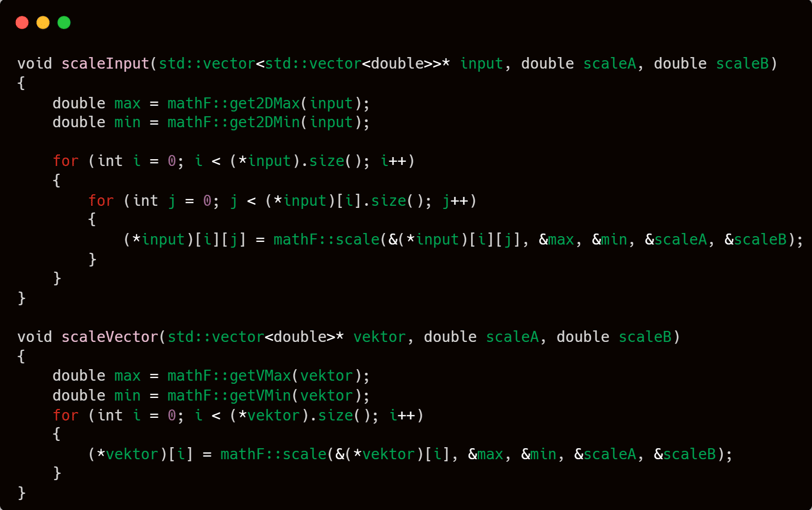
Moving on to the next two functions: scaleInput and scaleVector.

These functions serve as high-level wrappers for the scaling operations you’ve already seen. While the previous functions like randomScale2D and randomScale3D were focused on applying scaling across randomly initialized weights or matrices, these two are more general-purpose.

scaleInput is typically used for preprocessing input data, especially before feeding it into the network. It ensures that the input values fall within a certain range, improving training performance and convergence.
scaleVector offers a flexible scaling option for a single vector, useful for a variety of use cases where normalization or bounded values are needed.

Both rely heavily on:

getVMax and getVMin to find bounds,
and then use scale() from mathF to remap each value.

In short:

These functions make scaling operations clean, modular, and reusable — crucial for clean architecture and effective data preprocessing.

Both functions serve the same purpose — mapping a vector or matrix to a specific range — but the key difference lies in their scope:

scaleInput operates on a 2D matrix, making it ideal for scenarios like normalizing entire datasets where each row is a sample and each column a feature.
scaleVector, on the other hand, focuses on a 1D vector, making it more suitable for things like:
- Adjusting output vectors,
- Normalizing bias values,
- Or any situation where you need to scale a single array of numbers.

💡 Potential Use Cases:

When to Use scaleInput:

Before training, to normalize features in a training set.
When loading raw data from a .csv and wanting to map all values to a defined range (e.g., 0,10, 1 or −1,1-1, 1).
When testing how range normalization affects model convergence speed.

When to Use scaleVector:

Adjusting output scores before applying softmax or sigmoid.
Rescaling evaluation metrics.
Scaling gradient values in optimization tweaks.

Even if you won’t demonstrate them now, understanding where they shine gives you the ability to fine-tune or debug models more effectively later.

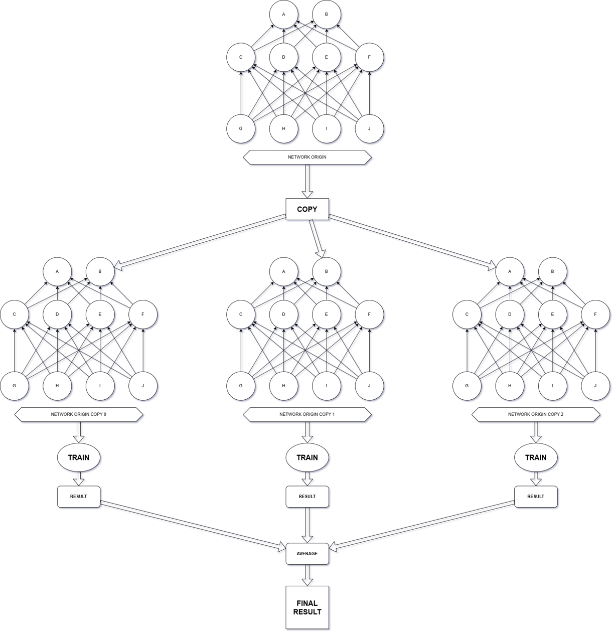
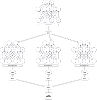
It's important to understand that during the training process of an artificial neural network, there's a technique often referred to as parameter averaging.
Whether this term is officially recognized or just something I coined myself—well, that’s up for debate. But the key point is: it actually works! Hahaha.

One essential aspect of parameter averaging is the use of parameters obtained from separate training processes.
For example, you start by creating two identical sets of parameters, including both biases and weights. These two models begin with the same initial values but are trained using different datasets or input sequences.
Once the training is complete, you calculate the average of corresponding bias and weight values from both models. This averaged result becomes your final trained output.
The concept is simple but effective, especially when aiming for stability or generalization in training outcomes.

💡 Additional Note: This technique is also applied in areas such as ensemble learning or federated learning, where separate models are trained independently and then combined using strategies like parameter averaging to enhance overall performance.

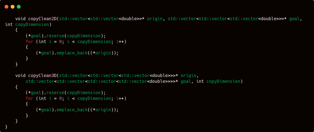
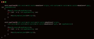
In order to obtain the averaged result, it's essential to start with two or more identical parameter sets. This is why I implemented two functions specifically for copying parameters.

The core idea is simple:

Duplicate a given parameter into a new container structure multiple times — say, x times.

The outcome is a matrix whose dimensionality is one level higher than the original parameter.
🔹 Example: If your original parameter is a 2D bias matrix and you need 4 such sets for averaging, you generate a 3D matrix, where:

The outermost dimension has a size of 4
Each inner element is a copy of the original 2D bias matrix

neuralNetwork.cpp

✅ The math functions are complete.
✅ The file organizer is wrapped up.
✅ The vector organizer is finalized.

Now, it's finally time for the main file of our artificial neural network to take the spotlight and shine in full glory.

This is where the core logic resides — the heart of the entire learning system. All the groundwork we've built so far comes together here.
As I’ve already mentioned, this is the heart of everything — the true core of the system.
This is where all the complexity and intricacies are concentrated.

It’s the nerve center — the place where the logic, architecture, and mathematical machinery of the neural network converge. Expect no shortcuts here; only raw structure and computation.

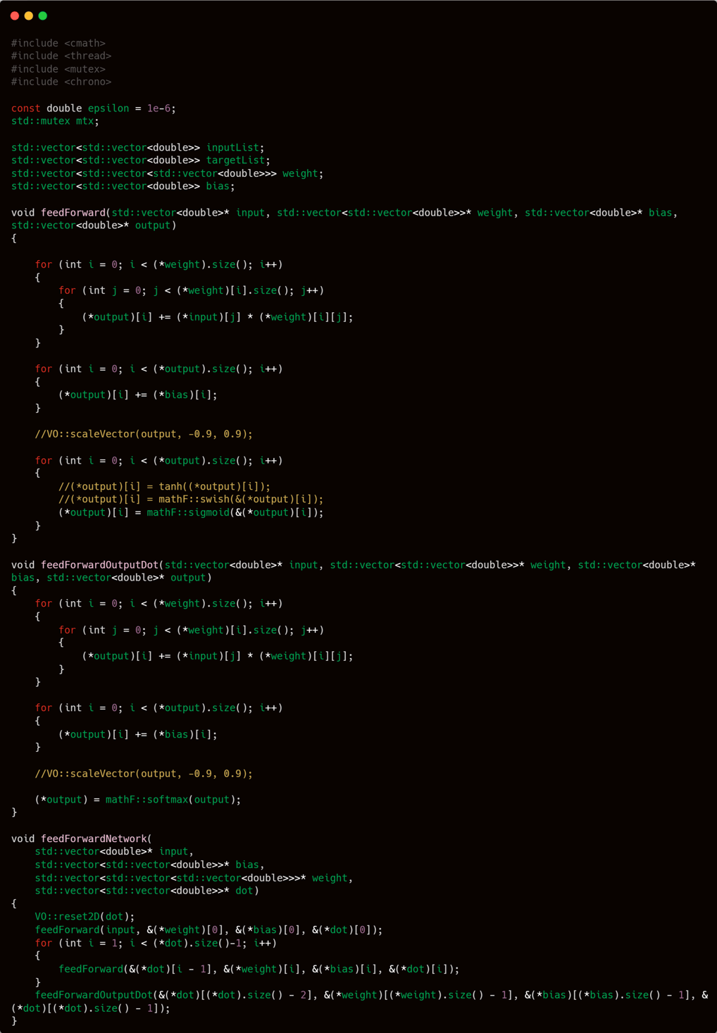
FEEDFORWARD -

I will divide the feedForward process into three distinct functions, each working through a nested structure — a function inside another function.

We will create three main functions:

feedForward – performs feedforward across all hidden layer neurons, then applies the chosen activation function to each hidden layer.
feedForwardOutput – performs feedforward only on the output layer, followed by its activation.
feedForwardNetwork – this function combines the two previous ones to execute feedforward through the entire neural network, ultimately generating the final output.

The workflow is simple and modular, allowing clear separation between hidden-layer processing and output-layer computation.

BACKPROPAGATION -

While feedForward is quite simple, the real challenge begins with backPropagation.
This phase is significantly more complex because it relies on the chain rule from calculus, which requires careful handling of derivatives across multiple layers.

No matter how complex it may seem, a deeper analysis reveals a distinct pattern in how backward propagation works in an artificial neural network.
I plan to take a slightly different approach in executing the backpropagation process.
So please pay close attention to the following explanation of my mechanism, as it lays the foundation for this new method.

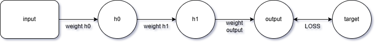
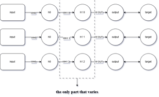
Let’s begin by imagining a simple neural network consisting of:

1 input neuron
2 hidden layers, each with 1 neuron
1 output neuron

This setup will help us focus on the basic flow of data and gradients through a compact network.

To update weightH0, we use the formula:

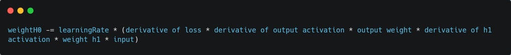
This represents the chain rule application propagating the error signal back from the output through hidden layer 1 to the input weight.

Now, let’s imagine adding 3 neurons to hidden layer 1, so that the network structure expands and now appears as follows:

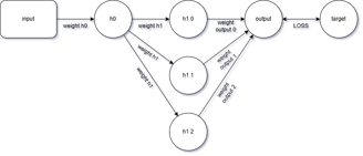
Upon closer inspection, you'll notice that backpropagation in this network occurs through 3 distinct paths.
In other words, the backward propagation process is essentially repeated 3 times, each along its own path through the network.

This highlights the multi-path nature of error flow in wider neural networks with multiple neurons in the same layer.

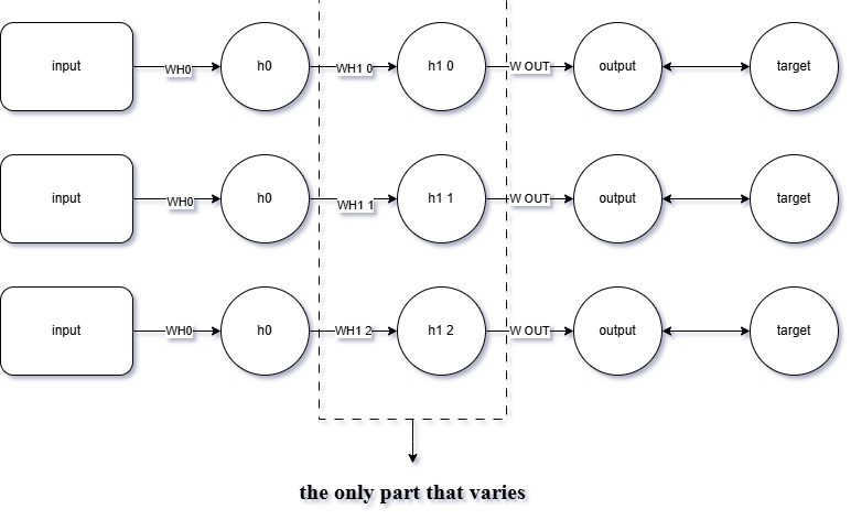
Since there are 3 different backward paths—caused by the presence of 3 neurons in hidden layer 1—
the update to the weight connecting the input to hidden neuron 0 will be computed 3 separate times, once per path.

Naturally, performing this mathematically for each path will cause the computational load to increase significantly,
especially when compared to the earlier network that had only a single path (before the 2 additional neurons were added to hidden layer 1).

This highlights one of the core challenges in scaling neural networks—as the width grows, so does the complexity of gradient flow.

The true issue isn’t the complexity itself—after all, no matter how complex it gets, that burden falls on the computer, not the programmer, whose job is simply to write the logic.

But when the challenge becomes one of massive computational demand, it turns into a business concern—resources, time, and efficiency become critical.
Stakeholders viewing this from a business standpoint may find it costly or unsustainable.

That’s why I developed the following solution.

🔁 Rather than taking this approach:

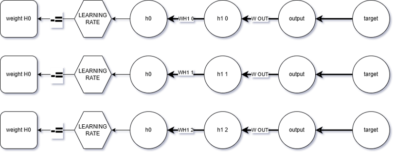
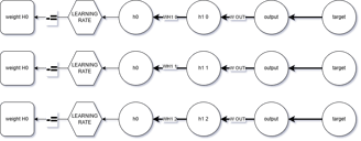
✅ It’s more efficient to proceed like this instead:

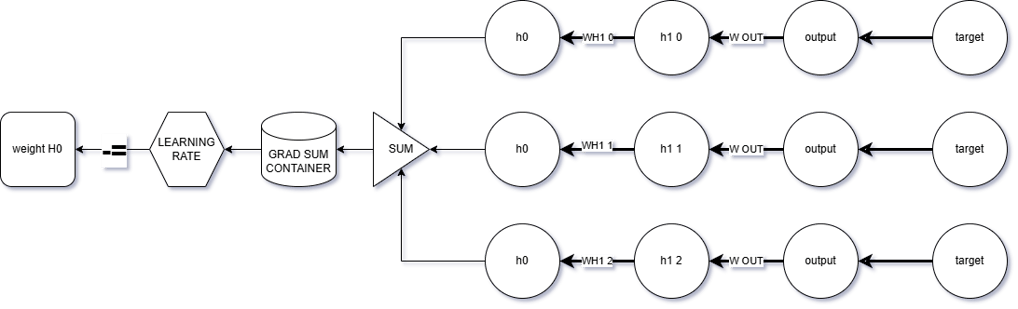
The approach I recommend is to store the accumulated gradient from the backpropagation path (just before it reaches the neuron containing the parameter to be updated — let’s call this dot x) inside a container.

Why do this?

Simple and efficient.

If dot x has multiple incoming weights, you can update them using the formula:
newParameter -= learningRate × gradSumContainer (at dot x) × input connected to that weight
✅ No need to re-traverse all paths.
If you wish to continue the chain rule back to earlier layers, you don’t have to multiply through the entire chain again.
Just multiply by the gradSumContainer, which already stores the cumulative gradient from deeper layers.
⚡ Less redundancy, more efficiency.

This method drastically cuts down on the computational load that would normally occur by repeatedly traversing back and forth from the frontmost layer all the way to the rearmost layer.

That’s enough theory —
Now, let’s step into the practical side of things.

💡 Time to build, implement, and test the ideas in action.

The plan is simple:

Create a vector container to store the gradients.
Populate this vector with the derivative values calculated at each dot.

🧩 Once all gradient-holding vectors are filled with their respective derivatives…
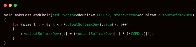
➡️ The next step is to create a dedicated function that applies the chain rule specifically to the output layer.

🔧 Inside this function:
Just multiply each dot’s value by the derivative of the loss,
then store that result back into the dot.

✅ This sets the stage for backpropagating cleanly through earlier layers.

That value we just calculated?
All that’s left is to multiply it by the corresponding input,
and boom — you’ve got what you need to update the output weights.

Once those two functions are ready,
you’ll need a third function — one that handles the accumulation of the chain rule in the hidden layers, as previously designed.

But keep in mind:
This function is not the same as the one that generates gradients for the output weights.

Why is it different?
Because when updating hidden layer weights, you're dealing with multiple intertwined paths, involving cross-multiplications between derivatives and weights.

🔧 So, this function will require a slightly more advanced mechanism to properly manage those complex interactions.

📣 To all readers:
I truly hope you've grasped the concept I explained earlier in the section about gradient sum containers. If not — go back and re-read it carefully.
Still confused?
📧📞 Feel free to reach out to me directly via email or phone. I’ll gladly walk you through it in person.
Why this matters? Because understanding this part is absolutely essential for following the next steps in the mechanism.

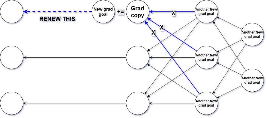
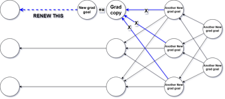
The third function we’re going to build is called: continueGrad.

Why that name?
Because this function’s role is to continue the derivative paths from the previous layers
and accumulate all those results into a coherent gradient flow.
It’s essentially the bridge that connects the gradient traces from deeper layers and propagates them further toward the front of the network.

To make things clearer,
take a look at the flowchart below –
it will help you visualize the process step by step and understand how everything connects.

To avoid repetitive manual calls to continueGrad in the main program logic,
it’s a good idea to wrap it inside another function.
This wrapper will act like a helper layer,
making your main code cleaner, simpler, and easier to manage.

All the core functions I’ve built so far are already enough to construct a simple neural network.
That means, in essence, the work is functionally complete ✅.

But in pursuit of better performance and more refined results,
I’ve also written a few extra helper functions — designed mostly for experimentation and further model exploration 🔬.

⚠️ Keep in mind:
These extra functions are not essential, and might not deliver the “wow” factor you expect.
However, if you're genuinely curious and wish to dive deeper,
feel free to contact me directly via email or phone.

💡 But again, don’t set your expectations too high—
these are just tools to help play around, not miracles.

Everything I’ve written so far consists of internal functions —
functions that do their job quietly behind the scenes, and are not meant to be called directly from the outside.

Now that all these essential building blocks are complete and ready,
it's time to move forward to the main functions —
the ones that will actually be called externally, or you might call them the public interface of the neural network.

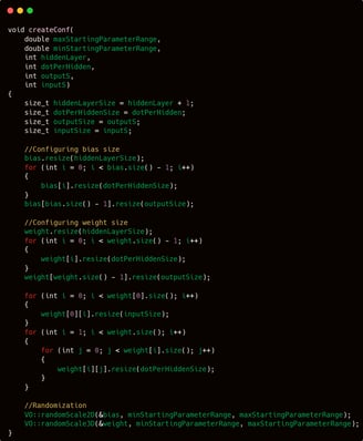
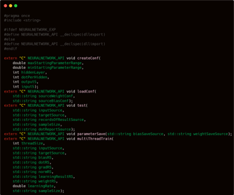
The first two externally callable functions are createConf and loadConf.
As their names imply, both are involved in defining the network’s initial structure.
The createConf function is used to build a completely new network from scratch according to user-defined settings,
whereas loadConf is used to load a pre-existing configuration from saved data.
These functions provide two distinct entry points—one for fresh model creation, and one for reusing existing configurations.

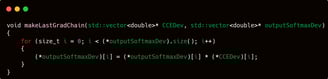
If you take a closer look, you'll notice that variables such as bias, weight, inputList, and targetList are all defined as global variables, at least within the scope of neuralNetwork.cpp.

If you're unsure where these variables were declared, I suggest revisiting the initial code sample I provided, particularly the first code I gave you from the neuralNetwork.cpp section.

The createConf function takes 6 parameters:

double maxStartingParameterRange
double minStartingParameterRange
int hiddenLayer
int dotPerHidden
int outputS
int inputS

The first two parameters, maxStartingParameterRange and minStartingParameterRange, are used to define the range within which the initial bias and weight values will be randomly generated.

The next two, hiddenLayer and dotPerHidden, control the structure of the neural network — allowing you to specify whether the network should be deeper (more layers) or wider (more nodes per layer).

Finally, outputS and inputS represent the number of output and input neurons, respectively — essentially determining the size of the input and output layers.

It is widely known that the parameters of an artificial neural network are initialized with random values. These values are generated using the functions randomScale2D and randomScale3D, which are defined within the VO namespace in the vectorOrganizer.cpp file. If you’re unsure or have forgotten where these functions are, feel free to revisit the "vector organizer" section for a refresher.

However, before assigning any values, the parameter structures must be reshaped to match the desired configuration. This is done by resizing the vectors using the resize function so that their dimensions align with the values provided to the createConf function.

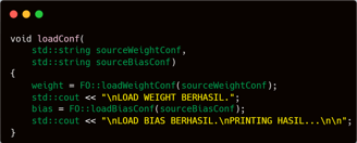
Setting up a configuration may involve several steps. However, reading a configuration is a different story—it's much simpler. All it takes is a single call to either loadBiasConf or loadWeightConf from the FO namespace, and the entire setup is instantly restored.

Training

Training — the phase where the neural network actually learns. Please follow along carefully, as this is one of the core components of the entire system.

The training phase will be divided into two closely related functions. While their connection might be predictable, it’s important to understand that both are part of a larger ecosystem — a structured set of functions that operate within one another to facilitate the training process effectively.

Typically, neural networks are trained using GPUs due to their high core count and parallel processing capabilities. However, since I’m working on a modest laptop without a dedicated GPU, my only viable option is to rely on multithreading with the CPU to simulate parallelism during training.

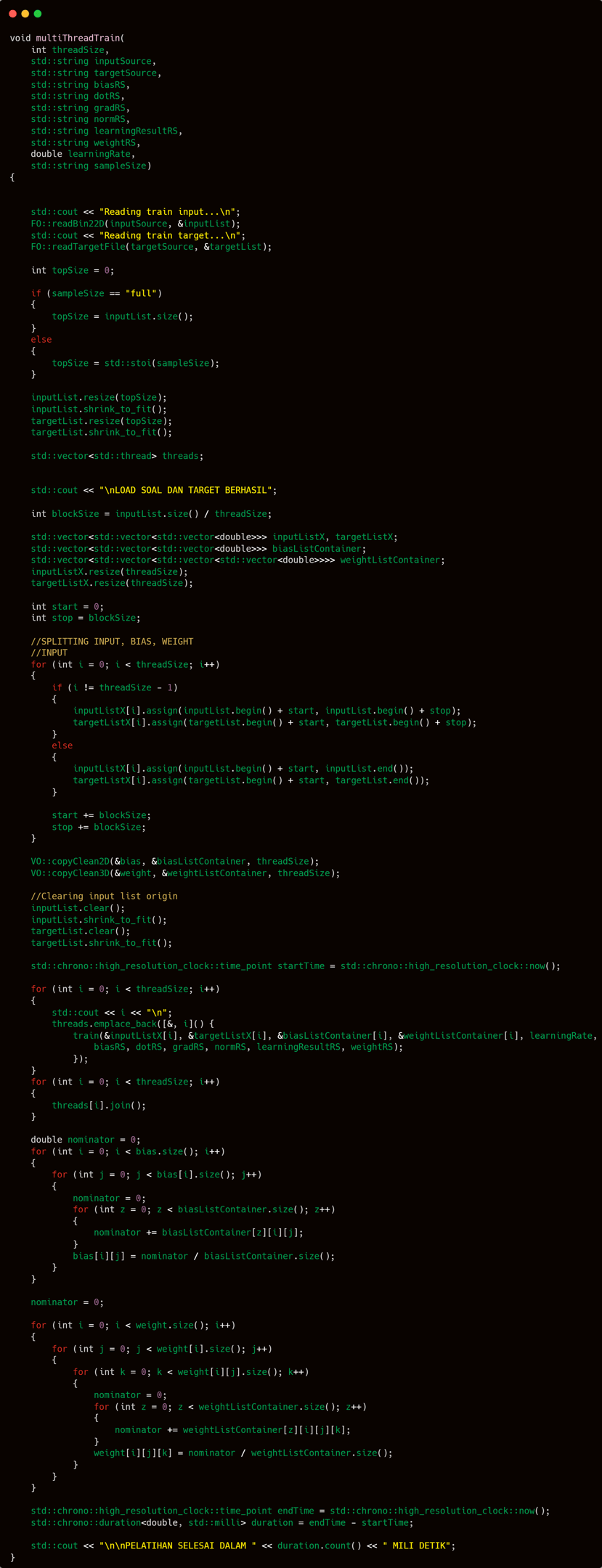
The training process is divided into two functions: train and multiThreadTrain. The multiThreadTrain function is publicly accessible and can be called externally, while train serves as an internal function. Instead of explaining both functions separately, I will describe the training mechanism as a whole—explaining how these functions work in tandem—so the overall process becomes clearer and easier to follow.

The training approach employed in this model is parameter averaging. In simple terms, this technique involves creating multiple clones of the neural network—each initialized with identical parameter states. These clones are then trained in parallel or separately. Once training is complete, the final model parameters are obtained by averaging the corresponding parameters across all trained clones.

The multiThreadTrain function acts primarily as an organizer, delegating the actual training tasks to the train function, which performs the core computations.
To fully understand how multiThreadTrain coordinates the training process

The multiThreadTrain function begins by loading the input and target data. Once the data is loaded, the next step is to trim the dataset—specifically the number of input-target pairs that will be used for training.
This trimming process is essential in cases where, for example, a trainer has 1 million training samples but wants to start by experimenting with only 500,000 of them.
After the trimming step, the leftover data and any unused memory are cleaned up to ensure efficient memory usage.
Technically, this wouldn't be a concern if I had access to a supercomputer—haha! But in any case, it's always good practice to clean up unnecessary memory usage.

The next step is to prepare multiple network copies needed to enable parallel training using CPU-based multithreading.
Here’s a breakdown of what happens at this stage:

The input dataset is split into several parts, with the number of splits matching the number of threads allocated for training.
For each thread, a separate clone of the weights and biases is created.
Don’t forget to initialize and prepare the vector<thread> which will be used to run training tasks in parallel.
Once everything is set up, the original inputList and targetList are cleared to free up memory, since the data has already been distributed to their respective locations.
The original weight and bias are preserved, as they will be used later to store the final averaged parameters after all threads complete training.

Once everything is fully prepared, it's time to begin the training.
Start the timer to measure performance, launch all threads to begin parallel training, and finally wait for all threads to complete by joining them.

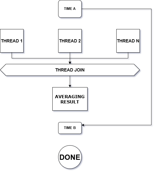
Once all parallel computations are completed, proceed as previously planned: calculate the average of each parameter to determine the final values that will be used in the model.
Next, start a new timer and measure the time difference between the start and end of training to determine the total duration. That concludes this phase..

From here on, the focus will shift to the inner workings of the training process that are executed by the multithreaded system.

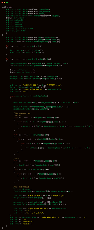
At its core, the train function operates with a very straightforward workflow. It takes in bias, weight, target, input, and learning rate as its primary parameters. Optionally, if you want to keep a training log, you can also provide file containers to store report data.
The process involves looping through each input entry, performing a feedforward step, followed by backpropagation, and repeating this sequence until the loop completes. That’s all—at least from a surface-level perspective.

But that is just the basic workflow, and we will now move into more detailed territory.

The training process begins with the creation of internal matrices: dot, grad, and a container for CCE (categorical cross-entropy) values. These are initialized directly within the train function rather than being passed in from the outside.
This design decision is based on efficiency. By declaring them internally, they are automatically cleaned up when the function ends—eliminating the need for manual memory management.
Additionally, each thread or training instance gets its own dedicated and isolated set of these variables, preventing unintended interference between processes.
Compared to externally defining these containers—managing their configurations and manually freeing their memory afterwards—this internal approach is significantly cleaner and more memory-efficient.

Once everything has been set up, the training process begins. A loop is created to iterate through each entry in the input list. For each input-target pair, the training steps—forward pass, backward propagation, and parameter updates—are executed in sequence. And with that, the training officially begins.

Before we go any deeper, keep in mind that the upcoming for loop will involve functions that have already been created earlier in this project. If you’re unsure about any of them, I strongly recommend reviewing my previous explanations—particularly those related to the training workflow. This is important, as I don’t intend to repeatedly go back and explain the same things again later on. Let’s move forward efficiently.

The first step inside the training for loop, which iterates through the input list, is calling feedForwardNetwork. This function executes the entire feedforward process, propagating the input forward through all the layers of the network until every neuron—including those in the output layer—is filled with the appropriate activation values.

Keep in mind that this for loop is the main one—it's the loop that iterates over every row of the input list. Therefore, whenever you see feedForwardNetwork or any other function using the index i, it's referring to the current input sample being processed by this outer loop:
for (int i = 0; i < (*inputListX).size(); i++)
This loop serves as the backbone of the training cycle, ensuring that each input-target pair goes through the full training step, one by one.

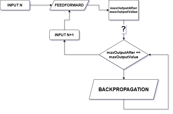
Once feedForwardNetwork finishes processing input[i], the next step is to define three critical variables:

oneTargetId: identifies which index in the target vector at position i holds the value 1 (i.e., the correct class in one-hot encoding).
maxOutputAfter: stores the output value (from the dot layer) corresponding to oneTargetId.
maxOutputValue: captures the highest value found among all output neurons at that step.

These variables play a key role in determining the depth and intensity of the backpropagation process for each input sample.

I’ll explain how these three variables are used and why they matter in practice a bit later. For now, make sure you understand their purpose—because they play a critical role in guiding how the backpropagation process will unfold.

Backpropagation is a process that adjusts parameter values by applying the chain rule backward through the network.

The main objective is to minimize the error between the predicted output and the correct target output.

For instance, if at row 20 the correct class is index 2, and the feedforward pass yields a value of 0.30 at output dot[2], then backpropagation aims to increase that value.

After one update, it might rise to 0.31, and with another update, it could reach 0.40. That’s the core idea behind how learning happens in this context.

Following that idea, my plan is to repeatedly apply backpropagation on training row x until the output value at the target index becomes the highest among all output values.

This is where maxOutputAfter and maxOutputValue become essential. They serve as benchmarks to decide whether backpropagation should continue, stop, or even be skipped entirely.

maxOutputAfter holds the value of the target class (where the one-hot target is 1), while maxOutputValue stores the highest value across all output neurons. The logic is simple: as long as maxOutputAfter is not equal to maxOutputValue, backpropagation should continue. In other words, we keep backpropagating until the target output becomes the highest among all outputs.

This method helps ensure that the model becomes confident in what data of class y should look like. On the flip side, if the model already makes the correct prediction even before any backpropagation, we can just skip it—since the model is already certain that input x corresponds to class y.

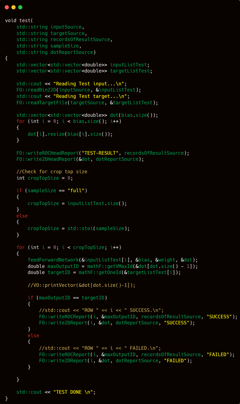
With the training phase completed, it is now time to implement the test function to assess the performance of the neural network.

In contrast to the relatively complex and intricate training process, testing is straightforward. The procedure involves trimming the input based on a predefined limit, iterating through each input row using a loop, performing feedforward on each, and recording the results. It's a simple and direct process.

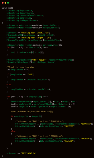
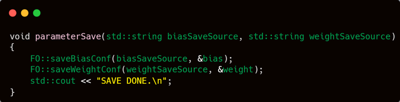
Similarly to the test function, the saveParameter function is straightforward. It is responsible for storing the parameter values in binary format. The core implementation of this saving mechanism is properly handled within the FO namespace. Thus, in the main routine, it simply involves invoking the saveBiasConf and saveWeightConf functions, followed by printing "SAVE DONE" to indicate completion.

All components have been completed. The final step is to adjust the header file (.h) for main.cpp or neuralNetwork.cpp. As previously explained, I will export only five functions and compile this project as a .dll to enable integration with other projects.

I’m going to test the training process of this program using a fraud detection dataset I found on Kaggle.

This dataset contains data about credit card transactions. There are more than 550 thousand records. Each record is, of course, anonymized for privacy. The task is to determine which transactions are fraudulent and which are not. From the task itself, it is already clear that the model to be built is a model for binary classification.

Actually, I have done many experiments to achieve optimal results. The experiments I did include adding the number of hidden layers, increasing the number of neurons per layer, finding the right combination between the number of hidden layers and neurons per layer, and finding the right activation function for the hidden layers. However, that process will not be documented and will not be shown because I feel that discussion already enters the fine-tuning realm and is not related to building a neural network library. Therefore, I will only share the final product files with readers for them to perform their own experiments.

The data that I will use for the practice is the fraud data I explained earlier. The data consists of around 550 thousand rows × 29 columns + 1 target column. I will use about 80 percent of the data for training and the remaining 20 percent for testing.

It should also be noted that I have done several experiments regarding the number of dots per layer, number of layers, activation functions, and so on. So what I will record is only how fast this program can run. There will be no report logging per iteration even though the logging function exists. I will only record the test prediction progress, because that log is needed to see how well the program predicts.

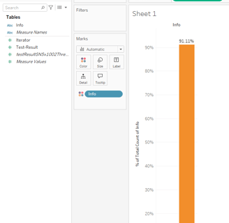
And this is the prediction accuracy percentage of the model shown in the video.

In conclusion, this project demonstrates how a neural network can be built entirely from scratch using C++, without relying on any external libraries, while still handling a large-scale dataset with a relatively complex architecture. Through the training and testing phases, the model has shown its capability in identifying potential fraud patterns and also served as a benchmark for evaluating the performance of a fully custom implementation.

This project not only serves as a technical exploration, but also reflects my commitment to deeply understanding and constructing artificial intelligence systems—from fundamental logic to advanced implementation.

If you're interested in learning more or have any questions about parts of the project that haven't been explained in full detail, feel free to reach out to me directly through the contact information provided on this website. I’ll be happy to discuss it further.